{ "title": "Understanding Shapley value explanation algorithms for trees", "description": "Game theoretic Shapley values have recently become a popular way to explain the predictions of tree-based machine learning models. This rise in popularity was made possible by new efficient algorithms. Here we examine how these algorithms work, and how they solve what is in general an NP-hard problem in linear time for trees.",
      "authors": [
        { "author": "Hugh Chen", "authorURL": "http://hughchen.github.io/", "affiliation": "Paul G. Allen School of CSE", "affiliationURL": "https://www.cs.washington.edu/"  },
        { "author": "Scott Lundberg", "authorURL": "https://scottlundberg.com/", "affiliation": "Microsoft Research", "affiliationURL": "https://www.microsoft.com/en-us/research/"  },
        { "author": "Su-In Lee", "authorURL": "https://suinlee.cs.washington.edu/", "affiliation": "Paul G. Allen School of CSE", "affiliationURL": "https://www.cs.washington.edu/"  }
      ] }
Understanding Shapley value explanation algorithms for trees
Game theoretic Shapley values have recently become a popular way to explain the predictions of tree-based machine learning models. This rise in popularity was made possible by new efficient algorithms. Here we examine how these algorithms work, and how they solve what is in general an NP-hard problem in linear time for trees.
One of the most popular machine learning model types are tree-based models. A 2017 survey of data scientists and researchers found that tree models were both the second and third most popular class of method (1). Although small tree models can be interpretable , most tree models are generally large and hard for humans to interpret.
1: The most popular data science methods according to a 2017 Kaggle survey (based on a total of 7,301 responses).
This article discusses how to explain tree-based models with Shapley values - a unique game-theoretic solution for spreading credit between features. First, we discuss how Shapley values can be applied to machine learning models (Section 1). Then, since exactly computing Shapley values for an arbitrary model is NP-hard , we discuss a recent exact algorithm focused specifically on tree models that runs in linear time (Section 2).
What is the goal of this article?
Given that there is a long history of model explanations going awry when users do not understand what an explanation means (e.g., p-values for linear models ), it is critical to have a broadly accessible explanation of Shapley values and how they are obtained for tree models to ensure that they are not misused. To this end, we aim to provide an easy to understand answer to two questions: 1.) What are Shapley values as used by popular package such as SHAP? 2.) How can we obtain Shapley values for trees? In particular, we focus on explaining a linear-time algorithm to explain trees in the SHAP package called Interventional Tree Explainer (this algorithm was first introduced and empirically evaluated in ).
1. Defining the feature attribution problem
In this section, we introduce the notion of feature attributions. Then, we introduce Shapley values and describe the ways in which they have been used to explain machine learning models, using an example with a linear model to motivate a specific extension of the Shapley values. With this formulation, we show how obtaining these Shapley values reduces to an average of Baseline Shapley values that can be thought of as explanations with respect to a single foreground sample (sample being explained that we will denote as \(x^f\)) and a single background sample (sample the foreground sample is compared to that we will denote as \(x^b\)).
1.1 The high level goal of feature attribution
The goal of feature attribution methods is to explain a model by assigning an importance value for each feature the model uses. In order to discuss the goal of feature attribution, it is useful to think about a linear model:
$$
f(x)=\beta_0 + \beta_1 x_1 + \cdots + \beta_d x_d
$$
Linear models are considered inherently interpretable because they summarize the importance for each feature with a scalar value where the importance (\(\phi\)) of a given feature (\(i\)) for a linear model (\(f\)) is:
$$
\phi_i(f)=\beta_i
$$
The attribution \(\phi_i(f)\) is known as a global feature attribution that explains the model as a whole. This is possible because features in a linear model are constrained to have a linear relationship with the model prediction, so a sufficient statistic to describe the relationship between any feature and the output of the model is the slope of that feature.
However, in many cases, it may be preferable to give a more individualized explanation that is not for the model as a whole, but rather for a specific sample's prediction (\(f(x^f)\)). For linear models, we could do so by returning an attribution of the following form:
$$
\phi_i(f,x^f)=\beta_i x^f_i
$$
The attribution \(\phi_i(f,x^f)\) is known as a local feature attribution that explains the model for a specific individual. Here, the attributions are easy to obtain because the relationship between \(x^f\) and \(f(x^f)\) is constrained to both be linear and consist only of marginal effects.
However, many easily interpretable models require making unrealistic assumptions (e.g., linear relationships in linear models, strictly marginal or pairwise effects in generalized additive models). Instead, if we use non-linear models that allow for complex interaction effects between variables, we can much better capture relationships in our data. For these models, summarizing non-linear effects with a single number (a global feature attribution \(\phi_i(f)\)) may not make sense, because we no longer have a slope. Instead, we can aim for local feature attributions (\(\phi_i(f,x^f)\)) that will explain the model's prediction for a specific individual. In order to do so in a principled manner, we can turn to the Shapley values.
1.2 Back to basics with Shapley values
Shapley values are a method to spread credit among players in a "coalitional game". We can define the players to be a set \(N=\{1,\cdots,d\}\). Then, the coalitional game is a function that maps subsets of the players to a scalar value:
$$
v(S):\text{Power Set}(N)\to\mathbb{R}^1
$$
To make these concepts more concrete, we can imagine a company that makes a profit \(v(S)\) that is determined by what combination of individuals they employ \(S\). Furthermore, let's assume we know \(v(S)\) for all possible teams of employees. Then, the Shapley values assign credit to an individual \(i\) by taking a weighted average of how much the profit increases when \(i\) works with a group \(S\) versus when he does not work with \(S\). Repeating this for all possible teams \(S\) gives us Shapley values:
$$
\overbrace{\phi_i(v)}^{\mathclap{\text{Shapley value of }i}}
=
\underbrace{\sum_{S\subseteq N\setminus\{i\}}}_{\mathclap{\text{All subsets w/o }i}}
\overbrace{\frac{|S|!(|N|-|S|-1)!}{|N|!}}^{\mathclap{\text{Weight }W(|S|,|N|)}}
(
\underbrace{v(S\cup\{i\})-v(S)}_{\text{Profit individual }i\text{ adds}})
$$
Coalitional game
Subset \(S\)
Profit \(v(S)\)
\(\{\}\)
\(\{Ava\}\)
\(\{Ben\}\)
\(\{Cat\}\)
\(\{Ava,Ben\}\)
\(\{Ava,Cat\}\)
\(\{Ben,Cat\}\)
\(\{Ava,Ben,Cat\}\)
Shapley values
\(\phi_{Ava}(v)\)
0
\(\phi_{Ben}(v)\)
0
\(\phi_{Cat}(v)\)
0
No credit.
2: Shapley values for a company that makes a profit \(v(S)\) based on it's three prospective employees \(Ava\), \(Ben\), and \(Cat\).
Shapley values are an excellent way to give credit to individuals in a coalitional game. In fact, they are known to be a unique solution to spreading credit as defined by the following three desirable properties (all of which hold for any coalitional game, as can be seen in 2):
Local Accuracy/EfficiencyThis property suggests that the units associated with the Shapley values are in terms of the coalitional game. For instance, when we adapt them to explain machine learning models, the explanation will be in units that correspond to the model's output (e.g., probability space, etc.) : The sum of Shapley values for all employees adds up to the profit with all employees minus the profit with no employees (2A-2D):
$$
\sum_{i\in N} \phi_i(v)=v(N)-v(\{\})
$$
Consistency/MonotonicityThis property is particularly important and implies that the Shapley values for features are ordered appropriately.: If an employee \(i\) always increases company \(v_1\)'s profit more than they would company \(v_2\) for all possible teams of employees, then \(i\)'s attribution for \(v_1\) should be greater than or equal to their attribution in \(v_2\) (2C vs. 2B):
$$
v_1(S\cup {i})-v_1(S)\geq v_2(S\cup {i})-v_2(S) \forall S \implies \phi_i(v_1)\geq \phi_i(v_2)
$$
Missingness: Employees \(i\) that don't help or hurt the company's profit must have no attribution (2D):
$$
v(S\cup {i})=v(S)\forall S\implies \phi_i(v)=0
$$
1.3 Adapting Shapley values to explain machine learning models
Shapley values are an optimal solution for allocating credit among players (\({1,\cdots,d}\)) in a coalitional game (\(v(S)\)). However, our goal is actually to allocate credit among features (\(x:=\{x_1,\cdots,x_d\}\in\mathbb{R}^d\)) in a machine learning model (\(f(x)\)) which is generally not a coalitional game:
$$
v(S)\neq f(x)
$$
In order to use Shapley values to explain a model, our goal moving forward is to define a new coalitional game related to the model's prediction:
$$
v(S)=g(f,x)
$$
As a first step, we can explore how coalitional games differ to machine learning models by looking at a model that is a coalitional game: a model with binary features \(x_i\in(0,1)\)Where 1 indicates presence of a feature and 0 indicates absence of a feature.. For such a model, the most natural coalitional game is the function applied to a vector that is one if the feature is in the set \(S\) and zero otherwise:
$$
v(S):=f(z^S)\text{, where } z^S_i = 1\text{ if }i\in S\text{, }0\text{ otherwise}
$$
However, most machine learning models actually have continuous features. In order to explain a typical machine learning model, we have to define both the presence and absence of featuresMore precisely, we have to define a new coalitional game \(v(S)\) related to the model's prediction \(f(x)\) where the features in \(S\) are present and the remaining features are absent. This is analogous to the way players \(S\) in a game are considered present and the remaining players are considered absent..
Presence of a feature: Our goal is to obtain local feature attributions (\(\phi_i(f,x^f)\)), a vector of importance values for each feature of a model prediction for a specific sample \(x^f\). This means that if feature \(i\) is present, we can simply set that feature to its value in the foreground sample \(x_i^f\). The next step is to address the absence of a feature, which can be done in several ways.
1.4 Absence of a feature (masking)
One straightforward way to address the absence of a feature is to define a baseline \(x^b\) (i.e., the background sample). In this case, if feature \(i\) is absent, we can simply set that feature to be \(x_i^b\). Then the new coalitional game is:
$$
v(S)=f(h^S)\text{, where } h^S_i = x^f_i\text{ if }i\in S\text{, }x^b_i\text{ otherwise}
$$
This specific adaptation of Shapley values to machine learning models is called Baseline Shapley, and were shown to be a unique solution to attribution methods with a single baseline based on cost-sharing literature . However, the choice of the baseline is a complicated one, and many different baselines have been considered including an all-zeros baseline, an average across features, a uniformly distributed baseline, and more (, , , ) For an in-depth discussion of this concept and a comparison of several baselines for Aumann-Shapley values applied to explaining images see ..
a.) Model and sample being explained.
Linear Model:
\(\beta_1\)
2
\(\beta_2\)
-1
\(\beta_3\)
10
Explicand:
\(x^f_1\)
70
\(x^f_2\)
135
\(x^f_3\)
0
b.) Zero baseline.
Baseline:
\(x^b_1\)
0
\(x^b_2\)
0
\(x^b_3\)
0
Attribution:
\(\phi_1\)
140
\(\phi_2\)
-135
\(\phi_3\)
0
c.) Average baseline.
Baseline:
\(x^b_1\)
70
\(x^b_2\)
135
\(x^b_3\)
0.5
Attribution:
\(\phi_1\)
0
\(\phi_2\)
0
\(\phi_3\)
-5
3: Example illustrating the downsides of a single baseline for Shapley values. Feature 1 corresponds to height (inches), feature 2 is weight (pounds), and feature 3 is gender (0 is male, 1 is female). The first baseline is an all-zero baseline. The second is an average feature value baseline.
For masking, the Shapley values for a linear model are easy to compute:
$$
\begin{aligned}
\phi_i(f,x^f,x^b)&= \sum_{S\in C } W(|S|,|N|)(f(h^{S\cup i}) {-} f(h^{S}))\\
&= \sum_{S\in C } W(|S|,|N|)(\beta h^{S\cup i} {-} \beta h^{S})\\
&=\sum_{S\in C } W(|S|,|N|) \beta_i (x^f_i-x^b_i)\\
&= \beta_i (x^f_i-x^b_i)\\
\end{aligned}
$$
Note that \(\sum_{S\in C } W(|S|,|N|)=1\).
One downside of Baseline Shapley is that the choice of baseline is very influential to the resulting feature attributions. In 3, we can see that the choice of baseline heavily influences the resulting attribution value.
3b is the zero baseline. In this case, it appears that height and weight are quite important, however being male is not important at all. This is a bit counter-intuitive, because relative to being female, being male reduces the prediction for this individual. Put another way, we can consider a new model where \(x_3\) is 0 for female, rather than 1 for female. Then, an equivalent model would be \(y=2x_1-x_2-10x_3+10\). In this case, using the same zero baseline gives an attribution value of -10 instead of 0 for being male for the exact same model. Since the meaning of zero is often arbitrary for different variables, selecting it as your baseline can result in misleading attributions.
Alternatively, we could use a mean baseline as in 3c. Although the mean of a binary variable does not have a natural interpretation, the mean baseline is actually a reasonable choice of baseline for linear models when we use the interventional conditional expectation to define our coalitional game (more details in Section 1.5). For this baseline, we see that for an individual with average height and weight, the importance of their height and weight should be zero relative to an average individual. Furthermore, in comparison to the zero baseline, the attribution for gender with a mean baseline will be consistent across different representations of gender.
For linear models comparing to an average individual baseline is equivalent to comparing to the average populationFor an interventional conditional expectation. However, if the data has binary features the average individual can be confusing, because they would be half female and half male. Comparing to the average individual is even more unappealing for non-linear models where comparing to an average individual is not equivalent to comparing to the average population. Rather than use a single background sample (or baseline) we can instead use many background samples and handling missingness with a conditional expectation over an entire population. In the next section we will describe two approaches to incorporate background distributions to our coalitional game \(v(S)\) for a better definition of missingness.
1.5 Absence of a feature (conditioning)
Another natural approach to incorporate a background distribution to the coalitional game is with a conditional expectation. Instead of simply replacing "missing" features with a fixed value, we condition on the set of features that are "present" as if we know them and use those to guess at the "missing" features. If we define \(D\) to be the background (underlying) distribution our samples are drawn from, the value of the game is:
$$
v(S)=\mathbb{E}_D[f(x)|x_{S}]
$$
One caveat is that getting this conditional expectation for actual data is very difficult. Furthermore, even if you do manage to do so, the resulting explanations can end up having undesirable characteristics (more on this later). Because our goal is just to explain the model itself, an arguably more natural approach is to use causal inference's interventional conditional expectation:
$$
v(S)=\mathbb{E}_D[f(x)|\text{do}(x_{S})]
$$
The do notation is causal inference's do-operator . In words, we break the dependence between the features in \(S\) and the remaining features, which is analogous to intervening on the remaining features. The motivation behind this decision comes from which is also very close to Random Baseline Shapley in . Additionally, this is exactly the assumption made by Kernel Explainer and Sampling Explainer from the SHAP package.
Linear
Model
\(\beta_1\)
\(\beta_2\)
\(\beta_3\)
\(\beta_4\)
Covariance \(C\)
\(x_1\)
\(x_2\)
\(x_3\)
\(x_4\)
\(x_1\)
\(x_2\)
\(x_3\)
\(x_4\)
Foreground
Sample
\(x_1\)
\(x_2\)
\(x_3\)
\(x_4\)
\(\phi_1\)
\(\phi_2\)
\(\phi_3\)
\(\phi_4\)
Shapley Values (CE)
1
2
3
4
Shapley Values (ICE)
1
2
3
4
Independent variables.
4: Comparing two versions of Shapley values: conditional expectation (CE) and interventional conditional expectation (ICE). We make two simplifying assumptions:
The function is linear (\(f=\beta_1 x_1 + \beta_2 x_2 + \beta_3 x_3 + \beta_4 x_4\))
The data-generating distribution is multivariate normal (\(D\sim \mathcal{N}_4(0,C)\))
In general, computing the conditional expectation Shapley value is difficult; however, for a multivariate normal distribution the conditional expectation is easy to calculate. In addition, for a linear function the conditional expectation of the function equals the function applied to the conditional expectation (\(E[f(x)|x_S]=f(E[x|x_S])\)Note that this is not generally true. Only for affine functions.).
Computing Shapley values for a linear model is much easier than for other model classes Note that we assume features have zero mean in the following calculations.. This is how we compute them for 4.
First, to compute Interventional Conditional Expectation (ICE) SHAP values for a linear model, we can start with:
$$
\begin{aligned}
\phi_i(f,x)&= \sum_{S\in C } W(|S|,|N|)(\mathbb{E}_{D}[f(x)|do(x_{S\cup \{i\}})] {-} \mathbb{E}_{D}[f(x)|do(x_{S})])\\
&=\sum_{S\in C } W(|S|,|N|)(\mathbb{E}_{D}[\beta x|do(x_{S\cup \{i\}})] {-} \mathbb{E}_{D}[\beta x|do(x_{S})])\\
&=\sum_{S\in C } W(|S|,|N|) \beta (\mathbb{E}_{D}[x|do(x_{S\cup \{i\}})] {-} \mathbb{E}_{D}[x|do(x_{S})])\\
&=\sum_{S\in C } W(|S|,|N|) \beta_i x^f_i\\
&= \beta_i x^f_i\\
\end{aligned}
$$
Note that \(\sum_{S\in C } W(|S|,|N|)=1\).
Second, to compute Conditional Expectation (CE) Shapley values for a linear model, we assume the background distribution \(D\) is multivariate normal with zero mean and covariance \(C\), we can start with:
$$
\begin{aligned}
\phi_i(f,x)&= \sum_{S\in C } W(|S|,|N|)(\mathbb{E}_{D}[f(x)|x_{S\cup \{i\}}] {-} \mathbb{E}_{D}[f(x)|x_{S}])\\
&= \sum_{S\in C } W(|S|,|N|)(\mathbb{E}_{D}[\beta x|x_{S\cup \{i\}}] {-} \mathbb{E}_{D}[\beta x|x_{S}])\\
&= \sum_{S\in C } W(|S|,|N|)\beta (\mathbb{E}_{D}[x|x_{S\cup \{i\}}] {-} \mathbb{E}_{D}[x|x_{S}])\\
\end{aligned}
$$
Here, we know that \(\mathbb{E}_{D}[x|x_{S}]=C_{N\setminus S,S} C_{S,S}^{-1} x_{S}\).
In 4 we highlight tradeoffs between the conditional expectation and the interventional conditional expectation for a linear model. Comparing 4A to 4B, we can see that the correlation between variables will cause the CE Shapley values to be split between correlated variables. Although this may be desirable at timesFor example, if we are interested in detecting whether a model is secretly using a confounding variable, we may want CE Shapley values., it can feel unnatural as in 4D, where feature \(x_4\) is as important as feature \(x_3\) despite the fact the model explicitly does not use it.
Although both CE Shapley values and ICE Shapley values are meaningful, we will focus on ICE Shapley values moving forward for two reasons: 1.) ICE Shapley values are tractable to compute as opposed to CE Shapley values that require modelling many conditional expectations and 2.) ICE Shapley values more explicitly describe the model's behavior whereas CE Shapley values conflate the model's behavior with the correlation in the data.
1.6 Incorporating a background distribution
To compute \(\phi_i(f,x^f)\) we evaluate the interventional conditional expectation. However, this depends on a background distribution \(D\) that the foreground sample will be compared to.
One natural definition of the background distribution is a uniform distribution over a population sample (e.g., equal probability for every sample in a data set). With this background distribution, we can re-write the Shapley value as an average of Baseline Shapley values (which are analogous to masking missing features) :
$$
\phi_i(f,x^f)=\frac{1}{|D|}\sum_{x^b\in D}\phi_i(f,x^f,x^b)
$$
This follows because of the linear form of the Shapley equation and because the interventional conditional expectation has a very natural definition when the background distribution is a single sample \(x^b\) (\(D_{x^b}\)):
$$
\mathbb{E}_{D_{x^b}}[f(x^f)|\text{do}(x_{S})]=f(h^S)\text{, where } h^S_i = x^f_i\text{ if }i\in S\text{, }x^b_i\text{ otherwise}
$$
In other words, the interventional conditional expectation for a single background sample is the model prediction for a hybrid sample where the features in \(S\) are from the foreground sample and the remaining features are from background sample. This is as if we intervene on features in the foreground sample with features from the background sample (as in Section 1.4).
Define \(C\) to be all combinations of the set \(N \setminus \{i\}\) and \(P\) to be all permutations of \(N \setminus \{i\}\). Starting with the definition of Shapley values:
$$
\begin{aligned}
\phi_i(f,x^f)&= \sum_{S\in C } W(|S|,|N|)(\mathbb{E}_{D}[f(x^f)|\text{do}(x_{S\cup \{i\}})] {-} \mathbb{E}_{D}[f(x^f)|\text{do}(x_{S})])\\
&=\frac{1}{|P|}\sum_{S\subseteq P} \mathbb{E}_D[f(x^f)|\text{do}(x_{S \cup \{i\}})] {-} \mathbb{E}_D[f(x^f)|\text{do}(x_{S})]\\
&= \frac{1}{|P|}\sum_{S\subseteq P}\frac{1}{|D|}\sum_{x^b\in D} f(h^{S\cup \{i\}}) {-} f(h^{S})\\
&= \frac{1}{|D|}\sum_{x^b\in D} \frac{1}{|P|}\sum_{S\subseteq P} f(h^{S\cup \{i\}}) {-} f(h^{S})\\
&= \frac{1}{|D|}\sum_{x^b\in D} \underbrace{\sum_{S\subseteq C} W(|S|,|N|)f(h^{S\cup \{i\}}) {-} f(h^{S})}_{\text{Baseline Shapley value}}\\
&=\frac{1}{|D|}\sum_{x^b\in D}\phi_i(f,x^f,x^b)
\end{aligned}
$$
In summary, we show that the problem of obtaining \(\phi_i(f,x^f)\) With an interventional conditional expectation for the coalitional game. reduces to an average of simpler problems \(\phi_i(f,x^f,x^b)\) where our foreground sample \(x^f\) is compared to a distribution with only one background sample \(x^b\). Obtaining \(\phi_i(f,x^f,x^b)\) will prove to be an easy problem to tackle for tree models.
2. An algorithm to explain trees quickly and exactly
Now our goal is to tackle the simpler problem of obtaining Baseline Shapley values \(\phi_i(f,x^f,x^b)\) that are attributions for a single foreground sample and background sample. The examples in this section are all for a specific foreground sample, background sample, and tree specified in 5.
Tree Parameters Green links indicate the foreground sample goes down a particular split, red indicates the background sample does, and blue indicates both samples do. (Click nodes)
Node Variable:
Node Threshold:
5
Leaf Value:
5
Variable
Foreground Sample \(x^f\)
Background Sample \(x^b\)
\(x_1\)
\(x_2\)
\(x_3\)
5: Choose foreground sample \(x^f\), background sample \(x^b\), and tree parameters for the remainder of Section 2. This is the tree, foreground sample, and background sample that will be explained in the following examples.
2.1 Brute force
Based on the proof in Section 1.6, the brute force approach would be to compute the following:
$$
\phi_i(f,x^f,x^b)=\sum_{S\subseteq N\setminus\{i\}} \underbrace{W(|S|,|N|)}_{W}(\underbrace{f(h^{S\cup \{i\}})}_{\text{\textcolor{green}{Pos} term}} {-} \underbrace{f(h^S)}_{\text{\textcolor{red}{Neg} term}})
$$
The algorithm is then fairly straightforward:
Tree Parameters
Attribution Values
\(\phi_1\)
\(\phi_2\)
\(\phi_3\)
Foreground & background sample
\(x_1\)
\(x_2\)
\(x_3\)
\(x^f\)
0
0
10
\(x^b\)
10
10
0
\(h^S\)
\(h^{S\cup i}\)
Algorithm State
\(W\)
\(S\)
\(f(h^S)\)
\(S\cup{i}\)
\(f(h^{S\cup{i}})\)
1/3
1/6
1/6
1/3
def ite_brute(array xf, array xb, tree T, array N):
phi = [0]*len(xf)
for each feature i in N:
for each set S in powerset(setminus(N,i)):
hs = [xf[j] for j in N if j in S else xb[j]] # Hybrid samples
hsi = [xf[j] for j in N if j in union(S,i) else xb[j]]
fxs = T.predict(hs) # Predictions
fxsi = T.predict(hsi)
W = (len(S)!*(len(N)-len(S)-1)!)/(len(N)!) # Weight
phi[i] += W*(fxsi-fxs) # Calculate phi contribution
6: Brute force algorithm for the tree and samples specified in 5.
If we assume the computational cost of computing the weight \(W\) is constantWhich it will be if we memoize \(k!\) for \(k=1,\cdots,d\)., then the complexity of the brute force method is the number of terms in the summation multiplied by the cost of making a prediction (on the order of the depth of the tree). This gives \(O((\text{tree depth})\times 2^{d})\).
Then, in order to compute \(\phi_i(f,x^f,x^b)\) for all features \(i\), we have to re-run the entire algorithm \(d\) times, giving us an overall complexity of
$$
O(d\times (\text{tree depth})\times 2^{d})
$$
An exponential computational complexity is bad; however, if we constrain \(f(x)\) to be a tree-based model (e.g., XGBoost, decision trees, random forests, etc.), then we can come up with a polynomial time algorithm to compute \(\phi_i(f,x^f,x^b)\) exactly. Why is this the case? Well, looking at 6, we can see that even for explaining a single feature, the brute force algorithm may consider a particular path multiple times. However, to compute the Baseline Shapley value for a single feature, it turns out that we only need to consider each path once. This insight leads us to the naive algorithm in Section 2.2.
2.2 Naive Implementation
Before we get into the algorithm, we first describe a theorem that is the basis for this naive implementation.
Theorem 1: To calculate \(\phi_i(f,x^f,x^b)\), we can calculate attributions for each path from the root to each leaf and then sum them:
$$
\phi_i(f,x^f,x^b)=\sum_P \phi_i^P(f,x^f,x^b)
$$
To obtain \(\phi_i^P(f,x^f,x^b)\) for a given path \(P\), we define \(N_P\) to be the unique features in the path and \(S_P\) to be the unique features in the path that came from \(x^f\). Finally, define \(v\) to be the value of the path's leaf. Then, the attribution of the path is:
$$
\phi_i^P(f,x^f,x^b)=
\begin{cases}
0 & \text{if}\ i\notin N_P \\
\underbrace{W(|S_P|-1,|N_P|)\times v}_{\text{\textcolor{green}{Pos} term}} & \text{if}\ i\in S_P \\
\underbrace{-W(|S_P|,|N_P|)\times v}_{\text{\textcolor{red}{Neg} term}} & \text{otherwise}
\end{cases}
$$
Sketch of proof: Treat each path \(P\) in the tree from the root to each leaf as a separate model \(f^P(x)\) that returns the value of the leaf if that path is traversed by \(x\) or zero otherwise. This results in (\(\text{\# leaf nodes}\)) models that operate on disjoint parts of the input space, implying that our original model is equal to the summation of all of these path models:
$$f(x)=\sum_P f^P(x)$$
By the additivity of Shapley values,
$$\phi_i(f,x^f,x^b)=\sum_P\phi_i(f^P,x^f,x^b)$$
Then, we can simply calculate \(\phi_i\) for each path model. Since the path model is zero everywhere except for the associated path, we arrive to the solution in Theorem 1.
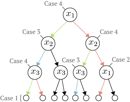
Given Theorem 1, we just need an algorithm to obtain \(N_P\) and \(S_P\) for each path, which can be done by traversing the tree. We will start by explaining the algorithm via an example:
7: Green paths are associated with \(\textcolor{green}{x^f}\), red paths are \(\textcolor{red}{x^b}\), and blue paths are associated with both.
In the naive algorithm, we maintain lists \(N_P\) and \(S_P\) as we traverse the tree. At each internal node (Cases 2-4) we update the lists and then pass them to the node's children. At the leaf nodes (Case 1), we calculate the attribution for each path. In 3, we see four possible cases:
Case 1: \(n\) is a leaf
Return the attribution from Theorem 1 based on \(N_P\) and \(S_P\)
Case 2: The feature has been encountered already (\(n_{feature}\in N_P\))
Depending on if we split on \(x^f\) or \(x^b\), we compare either \(x^f_{n_{feature}}\) or \(x^b_{n_{feature}}\) to \(n_{threshold}\) and go down the appropriate child
Pass down \(N_P\) and \(S_P\) without modifications because we did not add a new feature
Case 3: Both \(x^f\) and \(x^b\) are on the same side of \(n\)'s split
Pass down \(N_P\) and \(S_P\) without modifications because relative to \(x^f\) and \(x^b\) it's as if this node doesn't exist
Case 4: \(x^f\) and \(x^b\) go to different children
Add \(n_{feature}\) to both \(N_P\) and \(S_P\) and pass both lists to the \(x^f\) child
Only add \(n_{feature}\) to \(N_P\) and pass both lists to the \(x^b\) child
Tree Parameters
Foreground & background sample
\(x_1\)
\(x_2\)
\(x_3\)
\(x^f\)
0
0
10
\(x^b\)
10
10
0
\(h\)
Algorithm State
\(S_P\)
\(N_P\)
Attribution Values
\(\phi_1\)
\(\phi_2\)
\(\phi_3\)
def ite_naive(array xf, array xb, tree T):
phi = [0]*len(xf)
def recurse(node n, list np, list sp):
# Case 1: Leaf
if n.is_leaf: [Theorem 1]
for i in N:
if i in sp:
phi[i] += W(len(sp)-1,len(np))*n.value
elif:
phi[i] -= W(len(sp),len(np))*n.value
# Find children associated with xf and xb
xf_child = n.left if xf[n.feat] < n.thres else n.right
xb_child = n.left if xb[n.feat] < n.thres else n.right
# Case 2: Feature encountered before
if n.feat in np:
if n.feat in sp:
return(recurse(xf_child,np,sp))
else:
return(recurse(xb_child,np,sp))
# Case 3: xf and xb go the same way
if xf_child == xb_child:
return(recurse(xf_child,np,sp))
# Case 4: xf and xb don't go the same way
if xf_child != xb_child:
f_phi = recurse(xf_child,np+[n.feat],sp+[n.feat])
b_phi = recurse(xb_child,np+[n.feat],sp)
recurse(n=T.root,sp=[],np=[])
8: Naive algorithm for the tree and samples specified in 5.
Next we examine the computational complexity of computing \(\phi_i(f,x^f,x^b)\) for all features \(i\) using the naive algorithm.
For each internal nodes, the complexity is based on Cases 2-4. In the worst case, we need to check whether the current node's feature has been encountered previously by iterating through \(S_P\) and \(N_P\). Since these lists are of length \((\text{tree depth})\) in the worst case, each node incurs a linear \(O(\text{tree depth})\) cost.
For the leaf nodes, we compute the contributions for each feature (of which there are \(d\)). Then, computing the contributions for each feature requires checking whether the feature is in \(S_P\). This means that each leaf node incurs a cost of \(O((\text{tree depth})\times d)\) cost.
Putting this together, we get an overall cost of:
$$
O((\text{\# internal nodes})\times (\text{tree depth})) + O((\text{\# leaf nodes})\times (\text{tree depth}) \times d)
$$
In the next section we present two observations that allows us to compute \(\phi_i(f,x^f,x^b)\) for all features \(i\) in just \(O(\text{\# nodes})\) time.
2.3 Dynamic Programming Implementation
To improve the computational complexity of the straightforward naive algorithm, we can make two observations.
The first observation is that we can get rid of the multiplicative \((\text{tree depth})\) factor by focusing on what the lists \(S_P\) and \(N_P\) are used for. The first use is to check if a feature has been previously encountered. By replacing the lists with boolean arrays, we can check if a given feature has been encountered by a constant time access into the arrays. This means the internal nodes now incur a constant cost. The second use of \(S_P\) and \(N_P\) is to calculate \(|S|\) and \(|N|\) at the leaves. By maintaining integers that keep track of these values, the leaves no longer have to iterate through lists. This gets rid of the multiplicative \((\text{tree depth})\) factor for leaf nodes. These optimizations lead to a new computational complexity of:
$$
O((\text{\# internal nodes}) + O((\text{\# leaf nodes}) \times d)
$$
The second observation is that we can compute the attributions for all features simultaneously as we traverse the tree by passing \(\textcolor{green}{\text{Pos}}\) and \(\textcolor{red}{\text{Neg}}\) attributions to parent nodesAs a reminder, the \(\textcolor{green}{\text{Pos}}\) and \(\textcolor{red}{\text{Neg}}\) attributions correspond to the following terms in Theorem 1:
$$
\phi_i^P(f,x^f,x^b)=
\begin{cases}
0 & \text{if}\ i\notin N_P \\
\underbrace{W(|S_P|-1,|N_P|)\times v}_{\text{\textcolor{green}{Pos} term}} & \text{if}\ i\in S_P \\
\underbrace{-W(|S_P|,|N_P|)\times v}_{\text{\textcolor{red}{Neg} term}} & \text{otherwise}
\end{cases}
$$
. Before describing the algorithm in more detail, we first present a simple example that illustrates why we can pass up attributions.
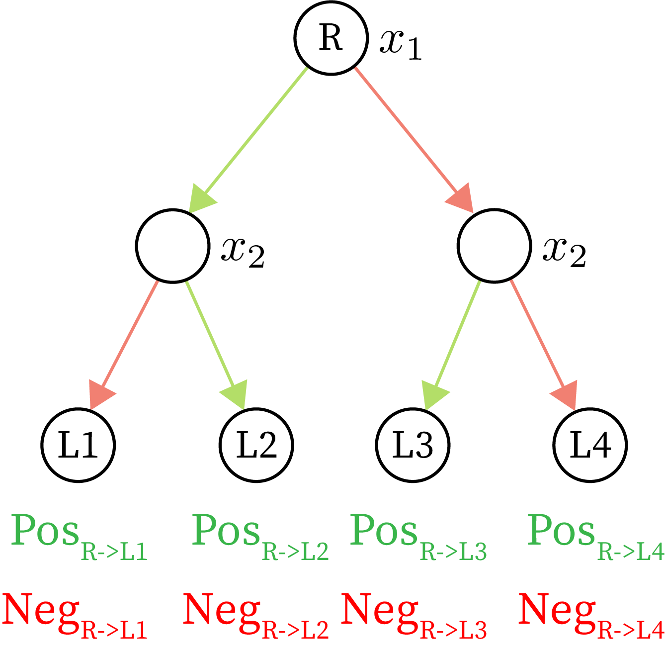
10 Example to illustrate collapsibility for features. Green paths are associated with \(\textcolor{green}{x^f}\) and red paths are associated with \(\textcolor{red}{x^b}\).
In 10, we can first observe that for each leaf, according to Theorem 1, there are only two possible values needed to compute the Baseline Shapley values (\(\textcolor{green}{\text{Pos}}\) and \(\textcolor{red}{\text{Neg}}\)). Based on the attributions for \(x_1\) we see that these \(\textcolor{green}{\text{Pos}}\) and \(\textcolor{red}{\text{Neg}}\) terms can be grouped by the left and right subtrees below \(x_1\). To generalize this example, we make the following observation:
Observation: We only add to the attribution for Case 4 nodes. For a specific Case 4 node \(n\), one child is associated with \(x^f\) and one child is associated with \(x^b\). If \(\phi_i(f,x^f,x^b)\) is initialized to zeros for all features, then, for each Case 4 node:
$$
\phi_{n_{feature}}(f,x^f,x^b)\mathrel{{+}{=}}\sum_{L\in \text{leaves}(x^f\text{ child})}\textcolor{green}{\text{Pos}_{R \to L}} + \sum_{L\in \text{leaves}(x^b\text{ child})}\textcolor{red}{\text{Neg}_{R \to L}}
$$
In words, we only consider \(\textcolor{green}{\text{Pos}}\) terms from all paths under the \(x^f\) child and \(\textcolor{red}{\text{Neg}}\) terms from all paths under the \(x^b\) child.
Therefore it is sufficient to add the \(\textcolor{green}{\text{Pos}}\) and \(\textcolor{red}{\text{Neg}}\) terms at a given node and pass them up to the parent to calculate the attributions for a parent node's feature. This aggregation of the \(\textcolor{green}{\text{Pos}}\) and \(\textcolor{red}{\text{Neg}}\) terms is the dynamic programming observation that allows each node to only need a constant number of operations.
Then, the dynamic programming algorithm computes the attributions for all features simultaneously (which gets rid of the multiplicative \(d\) factor for the leaf nodes):
Tree Parameters
Foreground & background sample
\(x_1\)
\(x_2\)
\(x_3\)
\(x^f\)
0
0
10
\(x^b\)
10
10
0
\(h\)
Algorithm State
\(S_C\)
\(N_C\)
Attribution Values
\(\phi_1\)
\(\phi_2\)
\(\phi_3\)
def ite_dynamic(array xf, array xb, tree T):
phi = [0]*len(xf)
def recurse(node n, int nc, int sc, array fseen, array bseen):
# Case 1: Leaf
if n.is_leaf:
if sc == 0: return((0,0))
else: return((n.value*W(sc,nc-1),-n.value*W(sc,nc)))
# Find children associated with xf and xb
xf_child = n.left if xf[n.feat] < n.thres else n.right
xb_child = n.left if xb[n.feat] < n.thres else n.right
# Case 2: Feature encountered before
if fseen[n.feat] > 0:
return(recurse(xf_child,nc,sc,fseen,bseen))
if bseen[n.feat] > 0:
return(recurse(xb_child,nc,sc,fseen,bseen))
# Case 3: xf and xb go the same way
if xf_child == xb_child:
return(recurse(xb_child,nc,sc,fseen,bseen))
# Case 4: xf and xb don't go the same way
if xf_child != xb_child:
fseen[n.feat] += 1
posf,negf = recurse(xf_child,nc+1,sc+1,fseen,bseen)
fseen[n.feat] -= 1; bseen[n.feat] += 1
posb,negb = recurse(xb_child,nc+1,sc ,fseen,bseen)
bseen[n.feat] -= 1
phi[n.feat] += posf+negb
return((posf+posb,negf+negb))
recurse(n=T.root,0,0,[0]*len(xf),[0]*len(xf))
10: Dynamic programming algorithm for the tree and samples specified in 5.
In 10 each node now only requires a constant amount of work. The computational complexity to compute \(\phi_i(f,x^f,x^b)\) for all features \(i\) with this algorithm is just:
$$
O(\text{\# nodes})
$$
2.4 Final considerations
Background distribution: Our original goal was to compute \(\phi_i(f,x^f)\). In order to do so, we compute \(\phi_i(f,x^f,x^b)\) for many references \(x^b\), resulting in a run time of:
$$
O(|D|\times (\text{\# nodes}))
$$
where \(|D|\) is the number of samples in the background distribution. In practice, using a fixed number of about 100 to 1000 references works well.
Further optimization: Explaining the tree for a specific foreground and background sample requires knowing where all hybrid samples go in the tree. Therefore we achieve the best possible complexity of \(\Omega(\text{\# nodes})\) for Baseline Shapley values. However, it may be possible to compute the attributions for many background samples simultaneously in sub-linear time in order to reduce the \(O(|D|\times (\text{\# nodes}))\) cost.
Ensembles of trees: Many tree based methods are ensembles (e.g., random forests, gradient boosting trees). In order to compute that attributions for these types of models, we can simply leverage the additivity of Shapley values and explain each tree and sum the attributions for each tree. This means that to explain a gradient boosting tree model, the computational complexity is:
$$
O((\text{\# trees}) \times |D|\times (\text{\# nodes}))
$$
Empirical evaluation: The goal of this article is understanding how these algorithms work, and not empirically evaluating them. For evaluation we refer readers to . In this article, we identify a way of assigning credit that comes equipped with a set of desirable properties (i.e., Shapley values) and show how to compute them exactly for trees with a tractable algorithm. This means that the credit allocation we obtain comes built in with many of the properties that empirical evaluation (often in the form of ablation tests) aim to measure (e.g., consistency).
Related Work
Methods in the SHAP package
It should be noted that there are a number of alternative methods that aim to estimate interventional conditional expectation Shapley values. A few of these methods include: Sampling Explainer, Kernel Explainer, and Path Dependent Tree Explainer. If you are explaining tree-based models, it may not be clear which one you should use. In this article we briefly overview a few of these the methods and compare them to Interventional Tree Explainer (ITE).
First, there are two model agnostic explanation methods in the SHAP package. The first is Sampling Explainer which is an implementation of Interactions-based Method for Explanation (IME) . This approach is based on sampling from all possible sets in order to estimate ICE Shapley values. The second is Kernel Explainer which is an extension of Local Interpretable Model-agnostic Explanations (LIME) to estimate ICE Shapley values. Both Sampling Explainer and Kernel Explainer are sampling based approaches that will converge to the same Shapley values ITE obtains. However, ITE is much faster in practice because it leverages the structure of the tree.
Second, in the SHAP package there is a method named Path Dependent Tree Explainer (PDTE) that is meant to obtain Shapley values for tree models specifically. PDTE approximates the interventional conditional expectation based on how many training samples went down paths in the tree, whereas ITE computes it exactly. The computational complexity of PDTE is \(O((\text{\# leaf nodes})\times (\text{tree depth})^2)\). In practice, PDTE can be faster than ITE, although it may depend on the number of references or the tree depth. The tradeoff is that the attribution values estimated by PDTE are biased away from interventional expectations by conditioning on parent nodes during the computation of the expected values.
Additional methods to explain trees
Two pre-existing methods to explain trees include Gain (Gini Importance) and Saabas. Both methods consider a single ordering of the features (as opposed to all possible orderings) specified by the tree they are explaining. Note that for an infinite ensemble of fully developed totally randomized trees Where a fully developed totally randomized tree is a decision tree where each node \(n\) is partitioned using a variable \(x_i\) picked uniformly at random among those not yet used upstream of \(n\), each node \(n\) has one child for each possible value of \(x_i\), and the construction of these trees is complete only when all variables have been used. and an infinitely large training sample, Gain is the mutual information between covariates and the outcome and Saabas gives the Shapley values . However, in practice trees are constructed greedily and both methods fail to satisfy the consistency axiom because they only consider a single ordering of the features.
Empirical Evaluation
In this article we do not empirically evaluate these methods, because evaluating interpretability methods can difficult due to the subjective nature of an explanation. Instead, we identify a way of assigning credit that comes equipped with a set of desirable properties (i.e., Shapley values) and show how to compute them exactly for trees with a tractable algorithm. This means that the credit allocation we obtain comes built in with many of the desirable properties that ablation tests aim to measure (e.g., consistency). That being said, provides an in-depth empirical comparison of many of these methods using a variety of ablation tests.
Acknowledgements
This material is based upon work supported by the National Science Foundation Graduate Research Fellowship under Grant No. DGE-1762114. Any opinion, findings, and conclusions or recommendations expressed in this material are those of the authors(s) and do not necessarily reflect the views of the National Science Foundation.